Plotting Earth Science Data
Vol. I
A guide to analyze and plot Earth Science data for Scientist of all programming skill levels
Prepared by: Michael Nguyen

Project Inspired by:
Dr. Donald Knuth - Literature Programming
Plotting Earth Science Data
Vol. I
A guide to analyze and plot Earth Science data for Scientist of all programming skill levels
Prepared by: Michael Nguyen

Dr. Donald Knuth - Literature Programming
Table of Contents
The beautiful world we live in is constantly changing and evolving. The media continuously reports and bring awareness of environmental issues such as global warming, climate change, pollution, and natural disasters. Huge debates over the casualty of environmental conditionings have led to massive protests, influenceability of political parties, adversely blaming the situation on natural disasters, and even challenging the creditability of scientists to predict and forecast disasters.

In some instances, society cannot distinguish the root of the problem and decouple one issue from another. As shown in the image above, our eyes naturally focus on the dog walking on the beach. The dog could be playing fetch, exploring its environment, and moving randomly along the shoreline. Secondly, our eyes only focus on the person holding on to the leash once a usual or unnatural event occurs. As a reference from the Cosmos-Epsiode 2, Neil deGrasse Tyson deploys this analogy to explain the difference between weather and climate. "Here's the difference between weather and climate. Weather is what the atmosphere does in the short term, hour-to-hour, or day-to-day. Weather is chaotic, which means that even a microscopic disturbance can lead to large-scale changes; that's why those 10-day weather forecasts are useless. The climate is the long-term average of the weather over a number of years. It's shaped by global forces that alter the energy balance in the atmosphere, such as changes in the Sun, tilts in the earth's axis, the amount of sunlight the earth reflects back to space, and the concentration of greenhouse gases in the air. A change in any of them affects the climate in ways that are broadly predictable."
Illustrated in the image above, "The dog meandering represents the short-term fluctuations that is the weather. It is almost impossible to predict what will attract the dog's interest next. It's difficult to know the results of the meandering because he is being held on a leash. We can't observe climate directly; all we see is the weather. The average weather over the course of years reveals a pattern." Neil deGrasse Tyson holding the leash is the person with the leash "represents the long-term trend which is climate." "Weather is hard to predict, but the climate is predictable. The climate has changed many times in the long history of the Earth, but always in response to the global force."
"Keep your eye on the Man, Not the Dog"
Neil deGrasse Tyson

For the full video reference: click the image above
The Earth science community is a vast multi-disciplined group of Environmental scientists, Biologists, Soil Scientists, Foresters, Agronomists, Meteorologists, Geophysicists, Marine biologists, Arborists, Geogrpahers, Oceanographers, Climatologists, Astronomers, and much more. As mentioned in the background section, climate and weather can be a complex and sensitive topics requiring evidence data to support theory, concept, or experimentation. While some scientists are only concerned with the soil's moisture, other researchers may be concerned with melting icebergs and rising sea levels. Furthermore, some scientists may only study the short-term effects on marine life populations, and others may be researching the devastation of civilization caused by cyclones and hurricane winds.
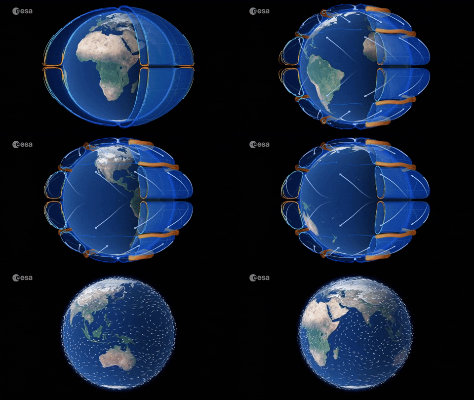
Despite the research topic, the desire for graphical representation, similar to the image above, is necessary to illustrate, represent, and communicate their message. Unfortunately, most of the community are not professional programmers, software engineers, or computer scientists. As a result, generating plots and animations is a daunting task and is often outsourced to individuals within the Geographic Information System (GIS) and Geospatial fields.
As an Electrical Engineer with over a decade of experience, I was in the same predicament. I was new to the Earth science field and wanted to plot my data to represent my theory and equations. I had done countless hours of market research and fell short of locating a versatile, simple, and well-supported tool. I was devasted to find that even a person with my creditial as a past software engineer of more than five years was incapable of finding a solution. On the contrary, individuals such as Biologist, Foresters, and Soil scientists must feel even more overwhelmed.
Consequently, I reviewed over 90 free software packages and 25 commerical license software to accomplish the task of analyzing earth science data, plots, and create animation. I had test trial some of these software packages. Most software packages are great for a single sole purpose, such as soil moisture but are limited to global temperature or wind speed. In addition, some software packages are in foreign languages making it difficult to translate into my native language, English. As a result, I took a different market research path to locate a programming language suitable for the task. Several contenders, such as C++, MATLAB, and Python, made the list; however, Python with cartopy provided the most versatile and simplest approach. In addition, cartopy is well supported by a large development team and has remained relevant since it was released in 2012.
As a scientist, it is my duty to contribute to the science community. Earth Science is a mixture of a diverse group within a niche area. The group is filled with driven individuals who want to improve the conditions for their children and generations so that they may step forward on this planet to leave the planet better than how it was left before their time. I hope this project finds helpful to scientists who have faced the same uphill problem that I once met. Regardless of the impact, the publication of this project will be beneficial for my personal gain as it contains all the lessons learned and procedures for future geospatial mapping and plotting projects.
The purpose of this project is to provide a guide to plot Earth Science Data for Scientists of all programming skill levels. This guide will include examples extracted from the Cyclone Global Navigation Satellite System (CYNSS) data product. In addition, the guide will cover data Level-1 and Level-2 data products published from the PODAAC. The programming language is chosen for this project is Python. Python is often used for beginners as it is one of the easier languages to learn due to its English-like syntax and organized structure. We determined that Jupyter Notebook Integrated Developmental Environment (IDE) is best suited for this project as it provides the data products for CYGNSS were obtained from a public domain from the PODAAC server. Maps and plots generated are based on 24-hour UTC information.
The data products for CYGNSS were obtained from the PODAAC server public domain. Maps and plots generated are based on 24-hour UTC information. Although the mission and theory for CYGNSS are challenging to understand, becoming familiar with the resources available and the background is a great way to learn any topic. The literature below is an excellent resource for this project. There is no need to go through thousands of pages at the moment. These resources will be explained in detail throughout this project.
PODAAC: Click here
CYGNSS Handbook: Click here
Other Useful References:
We live in a world that is constantly changing and evolving. Much like the natural laws of evolution, developmental software toolkits continually improve, providing new features and conducting route maintenance to fix bugs discovered from past generations while staying relevant to the latest trends and advances. As a result, publishing a step-by-step installation procedure for this project is futile and will be obsolete. Although this project aims to provide a guide for all programming skill levels, the list of software packages below has a long track record of being exceptionally thorough and detailed in their installation procedure. I recommend installing the software packages sequentially in the order given below.
I highly recommend installing Anaconda as it is an excellent tool in your arsenal. Anaconda is an open-source distribution of Python that includes a vast collection of packages and libraries for scientific computing, data analysis, and machine learning. Anaconda provides a convenient environment for managing and working with these packages, making it easy to get started with data analysis and machine learning projects. With Anaconda, you can create virtual environments, install packages with a single command, and manage your data science projects efficiently.
This project is developed in Jupyter Notebook and is an excellent tool for anyone who works with code, data, or documentation. Jupyter Notebook is an open-source web application that allows you to create and share documents that contain live code, equations, visualizations, and narrative text. It is a powerful tool enabling you to explore, prototype, and communicate your ideas effectively. With Jupyter Notebook, you can write and run Python coding language, making it a versatile tool for data analysis and scientific computing. Jupyter Notebook is an indispensable tool for your toolkit.
When programmers write code, they often need to analyze data that requires calculating complex algorithms to graph spatial coordinates accurately. However, writing this code from scratch can be time-consuming and generate errors. As a result, libraries are created to address the issue. Libraries are pre-written codes that programmers can import into their programs, which makes it easier to perform complex operations. For example, if a programmer wants to perform mathematical calculations in their program, they can import a math library with pre-written functions for doing these calculations. This saves time and makes the code easier to read and maintain. Therefore, programmers can write programs more efficiently, with fewer errors and more advanced features.
There are many ways to install libraries, but I highly recommend using the Anaconda command line interface for its ease of use and simplicity. Below is a list of libraries that are required. Each item on the list will contain a hyperlink to utilize the pip command approach to install the library. Below is a list of required libraries for this project subcategorized into Standard, netCDF, Mapping/Plotting, and Animation related:
4.3.1 numpy Purpose: Library contains Mathematic functions used for the field of Science and Engineering.
Installation Guide - PIP Shortcut: pip install numpy
4.3.2.1 netCDF4 Purpose: Library contains read/write functions for Version 4 and read/write HDF5 netCDF files.
Installation Guide - PIP Shortcut: pip install netCDF4
4.3.2.2 xarray Purpose: Alternative netCDF library. Library contains read/write functions for Version 4 and read/write HDF5 netCDF files.
Installation Guide - PIP Shortcut: pip install xarray
4.3.3.1 cartopy - Purpose: Library contains functions yused for geospatial data processing in order to produce maps and other geospatial data analyses.
Installation Guide PIP shortcut: pip install cartopy
4.3.3.2 cartopy.gridliner - Purpose: Library contains functions used to specify lat/lon grids axis based on World Geodetic System (WGS84) coordinate system.
(Installation is completed with 4.3.3.2)
4.3.3.3 cartopy.feature: (Installation is completed with 4.3.3.2) - Purpose: Library contains functions used to easily add map features of land, ocean, etc.
(Installation is completed with 4.3.3.2)
4.3.3.4 Matplotlib - Purpose: Extends some matploblib capabilities to plot cartopy projections and transform points. matplotlib.rcParams is increased to ensure that animation does not drop frames. This increases the default size for an animation. For more information click the following link: click here
Installation Guide: PIP Shortcut: pip install matplotlib
4.3.4.1 matplotlib.animation - Purpose: Library contains functions to create live animation from plots.
(Installation is completed with 4.3.3.4)
4.3.4.2 Matplotlib.FuncAnimation - Purpose: Library contains function for making animation and repeated loops.
(Installation is completed with 4.3.3.4)
4.3.4.3 Ipython.display - Purpose: Library contains functions to handle displaying plot, graphs, maps in Jyputer html format.
Installation Guide PIP Shortcut: pip install ipython
4.3.4.4 matplotlib.markers - Purpose: Library contains functions to designate specific markers to plot CGYNSS data products.
(Installation is completed with 4.3.3.4)
Jupyter Notebook has several advantages over other IDEs regarding literate programming (Dr. Donald and Dr. Jones).The main advantage of Jupyter Notebooks is that it allows for interactive coding. Software code runs and can be segmented and modified via cells in real-time, making it ideal for exploring data and experimenting with code. Additionally, Jupyter Notebooks provide a mix of code and markdown cells, allowing for clear and concise explanations of the code and making it easy for others to understand your thought process. Jupyter Notebooks also support Python, making it versatile for various data science and scientific computing projects. The following topics covered in this section are the fundamental basis of Jupyter for this project and will help to overcome the steep learning curve. The information below is obtained from Jupyter Notebook. I personally cherry-picked the topics below to expedite the learning curve.
Jyputer IDE is a server-based IDE that provides a web-based interface for working with programming code. The server can be run on your local machine, allowing multiple web pages to be open and running code individually segmented by cells. Jupyter IDE can be accessed using Anaconda to launch the notebook server. Afterward, the server will open a default web browser to the web application client with a default URL transcribed such as 'http://localhost:' or http://127.0.0.1:. These URLs depend on your network's local setting, and it is essential to understand that Jyputer does not send the data publically to the open web. The server is run locally on your machine and is self-contained.
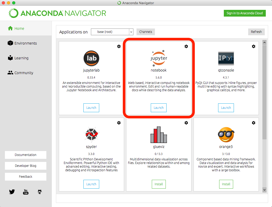
Using Anaconda Navigator launch Jupyter Notebook, as shown in the image below.
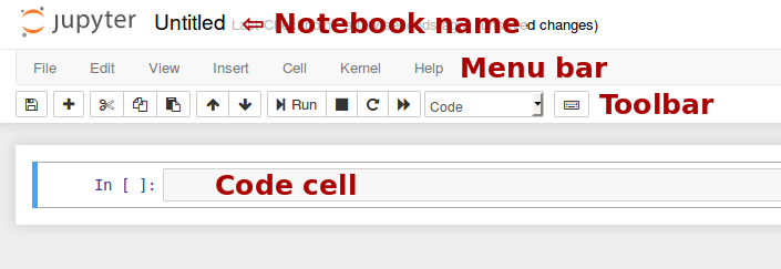
The image below shows that the web application client should display the Notebook dashboard. Understanding the Dashboard user interface before making any changes to the files or settings is very important. Below in red text are the locations for the Notebook name, Menu Bar, Toolbar, and Code cell.
After being familiar with the user interface, lets try to create a notebook file. Shown in the image below is a method to create a new file.
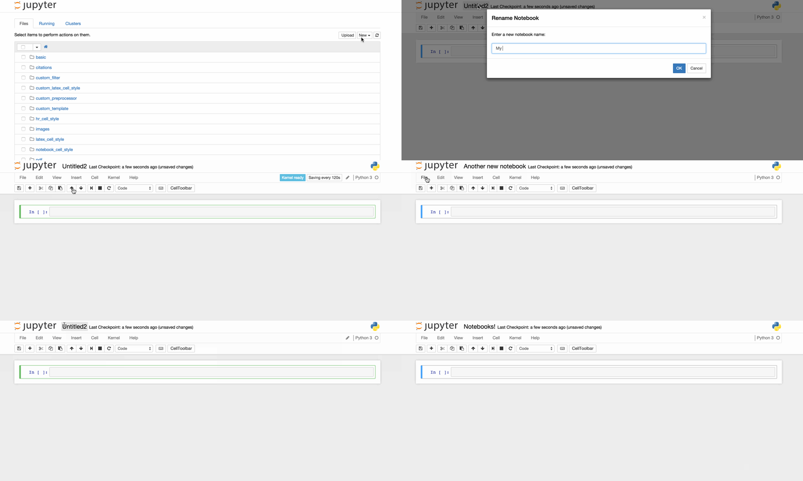
Click "File" on the Menu Bar and select "Save as.." and a Save as window should appear showing the current directory. Save the file into a desired directory or default directory. Please note the notebook file will need to be opened through the web application client and will require the developer to browse to the saved directory.
As shown in 5.3, the Jupyter Notebook code runs on individual cells. It is essential to become familiar with the steps to insert a cell. There are two options to insert a cell, insert a cell above or below the current cell.
Click "Insert" on the Menu Bar and select "Insert Cell Above" for the above option or select "Insert Cell Below" for the below option.

In some instances, the developer may want to remove the cell. In this case: Click "Edit" and select "Delete Cell"
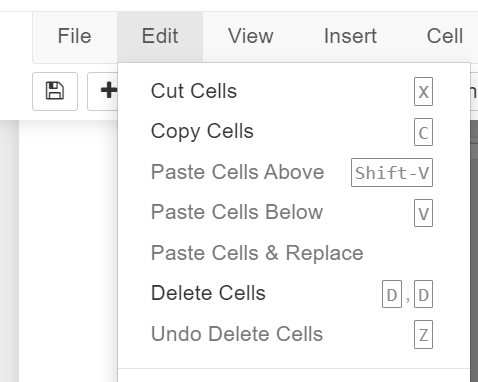
Jupyter Notebook is structured by three different types of operations: 1. Code cell, 2. Raw cell, and 3. Markdown cell.
A code cell allows the programmer to edite and write new code with full syntx highlighting and tab completion. By default, the cell is set in code cell mode with the kernel set to the IPython setting to execute Python code.
Raw cells provides provides the user a location to output directly in raw text. These cells are not evaluated by the kernel. As a result, we will raw cell to display sample code in this project. An example of Raw cell will be demonstrated in section 6.1.
By default, Jyputer set cells in the code mode. The code cell must be reconfigured to markdown to access this structure type. The following instruction is to change the cell type to markdown:
Click "Cell" on the Menu Barn, hover over "Cell type", and select "Markdown"
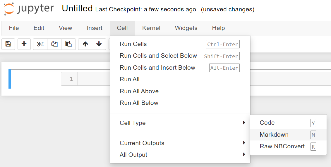
Markdown is a feature in Jyputer that allows the user to document the programming. In fact, the majority of this project is written in markdown mode to explain the project and procedures effectively. Below are some useful links to explain this powerful feature.
Other Useful References:
Jyputer Notebook allows the developer to access commands using the toolbar. Additionally, commands can be executed using keyboard short cut. I recommend becoming familiar with keyboard shortcut keys as it will improve the developmental workflow. Below are commonly used Jupyter Notebook Shortcut keys:
Execute/run the current cell and show any ouput. It is the same as Clicking the "Run" on the toolbar.
Enter the cell to make editification.
Save the Notebook and create a checkpoint.
For a complet list of shortcut keys, Click "Help" on the Menu Bar, and select "Keyboard Shortcuts"

Python is a popular and versatile programming language with many advantages over other programming languages. The programming language is simple and has readable syntax, making it easy to learn and use. Additionally, Python has a vast and active community of developers who contribute to many libraries and tools that can be used for various tasks, including scientific computing, data analysis, web development, and machine learning. Python also supports multiple programming paradigms, including procedural, functional, and object-oriented programming, making it flexible and adaptable to different project requirements. Moreover, Python has an extensive standard library that provides a range of useful functionalities, such as file I/O, networking, and regular expressions. Overall, Python is an excellent choice for beginners and professionals alike, as it is easy to learn, flexible, and has a broad range of applications.
The earth science community contains professionals of all skill sets, with people with minimal programming experience and others with 30 years+ as software developers within the industry. Because of the vast range of experience, the scope of this section is to only cover the basics of Python language for this project enough to understand the project successfully. As a programmer with 10 years+ of related experience in software, programming is similar to playing sports, and it will only get better when one puts in the time and practice. Also, covering four undergraduate semester programming courses for this project is unrealistic. Therefore, the approach only covers the essential topics related to this project and keeps those new to programming manageable. For those who are experienced programmers, feel free to skip this section. Below are some helpful links to learn Python. This section will cover the following topics:
Useful Links:
The best method to learn programming is to dive right in. Below is python code that can be copied and pasted into the code cell below. Once pasted in the cell below, click "Run" in the toolbar above or use the keyboard shortcut key Ctrl+Enter.
The print command in python is used to output a statement. Copy the bold text below and paste it into the code cell below to try the code.
Note: The cell below is configured as a Raw cell. Moreover, the cell below the Raw cell is the Code cell. A sample print command code is displayed in the Raw cell. Copy the text from the raw cell and paste the text into the code cell. Afterward, run the code inside the code cell, and you should see the print statement. Please experiment with the string of characters 'Hello World' as it can be modified to characters you like.
print ('Hello World')
The comment command in python is used to ignore the entire line of code. Programmers use the comment statement to debug their software and comment on their code. Copy the text below, paste it into the code cell below, and run the code.
Note: The cell below is configured as a Raw cell. Moreover, the cell below the Raw cell is the Code cell. A sample print command code is displayed in the Raw cell. Copy the text from the raw cell and paste the text into the code cell. Noticed the additional hashtag character '#' in front of the print command. Python recognizes this symbol as a comment code; therefore, no output or print statement will be displayed. Programmers use comments to temporarily remove a line of code or provide comments on the code.
#print ('Hello World')
The if statement is utilized throughout this project. The if statement is a logical argument and allows a code segment to be run based on a condition. Please see the sample code and syntax below.
Note: The cell below is configured as a Raw cell. Moreover, the cell below the Raw cell is the Code cell. A sample print command code is displayed in the Raw cell. Copy the text lines 1-8 from the raw cell, paste the text into the code cell, and run the code. This if statement code example provides great insight into the syntax for python. Noticed that under each if statement, the print code is spaced by a tab. Python programming recognizes these tabs, which makes them unique in organizing the if loop statement.
if condition:
do somethingx = 1 y = 2 if x == 1: print ('x') if y == 2: print ('y')
x = 1
y = 2

if x == 1:
	print ('x')

if y == 2:
	print ('y')
x
y
As described in section 4.3, this project will utilize various libraries functions call to plot/graph data points. Below is the execution code to import: numpy, netCDF, xarray, cartopy, matplotlib, and IPython libraries.
Note: Select the code cell below and run the code. If an error occurs, please refer to section 4.3 to verify that libraries install correctly.
import numpy as np

from netCDF4 import Dataset
import xarray as xr

import cartopy.crs as ccrs
from cartopy.mpl.gridliner import LONGITUDE_FORMATTER, LATITUDE_FORMATTER
import cartopy.feature as cfeature
import matplotlib.pyplot as plt

import matplotlib.animation as animation
from matplotlib.animation import FuncAnimation
from IPython.display import HTML
import matplotlib
matplotlib.rcParams['animation.embed_limit'] = 8**128
NetCDF (Network Common Data Form) files are commonly used in Earth science to store and share multidimensional scientific data, such as atmospheric and oceanographic data. These files provide a standardized format that allows scientists to easily exchange and analyze data across different platforms and software packages. netCDF files can contain a wide range of information, including metadata, spatial and temporal coordinates, and data values. This makes them an essential tool for scientists studying climate change, weather patterns, and other Earth science phenomena.

The organization standardizing netCDF file format is UNIDATA University Corporation, located in Boulder, CO. The company's core goal is to be the center for sharing, accessing, and data for visualization and analysis relating to geoscience. Furthermore, the standardization for NetCDF file format is funded by the National Science Foundation (NSF) and has been supported by educational and research institutions for over 30 years. netCDF data format is a standard file that various software applications can view.

Although Unidata University Corp standardizes netCDF file format, the collaboration with NASA's Earth Observing System Data and Information System (EOSDIS) has made the netCDF readily available to the earth science community. NASA EOSDIS is designed as a distributed system to distribute earth science data. NASA's Earth Science Data Systems (ESDS) Program oversees the life cycle of NASA's Earth science data from acquisition through processing and distribution. The primary goal of ESDS is to maximize the scientific return from NASA's missions and experiments for research and applied scientists, decision-makers, and society at large.
ESDS data systems and science products continuously evolve through a combination of competitive awards and sustained and strategic investments in open data, international and interagency partnerships, and a set of standards that ensure consistency and interoperability. Since 1994, Earth science data have been free and open to all users for any purpose, and since 2015, all data systems software developed through research and technology awards have been made available to the public as Open Source Software (OSS). ESDS falls within the purview of the Earth Science Division (ESD) under the Science Mission Directorate (SMD) at NASA Headquarters.
The EOSDIS deploys major facilities throughout the United States, referred to as Distributed Active Archive Centers (DAACs). These 10+ DAAC facilities process, achieve, document, and distribute data from NASA's past and current Earth-Observing Satellites and field measurement programs. Each DAAC is segmented into a particular expertise or discipline. For example, the Alaska Satellite Facility (ASF) DAAC is the custodian for Synthetic Aperture Radar (SAR) disciplines; the National Snow and Ice Data Center (NSIDC) DAAC is the custodian for Snow, sea ice, glaciers, ice sheets, frozen ground, soil moisture, climate interactions, etc. disciplines; the Ocean Biology DAAC (OB.DAAC) is the custodians for ocean color, sea surface temperature, sea surface salinity disciplines; etc.
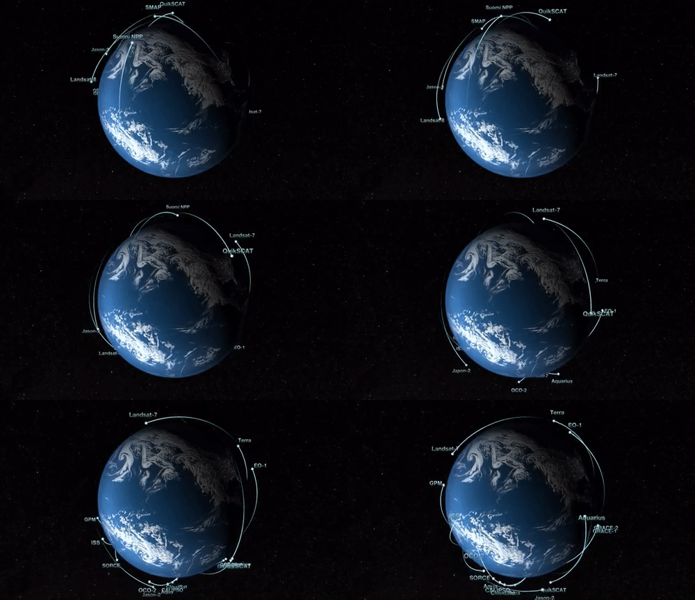
Uncovering the earth's mystery is a complicated and complex task requiring support from scientists of all backgrounds. NASA realizes that studying the earth is an essential mission as it is detrimental to the existence of life. As shown in the image below, NASA has launched many satellites in an effort to study the earth. Additionally, NASA published a graphical simulation of EOS Satellites orbiting earth.
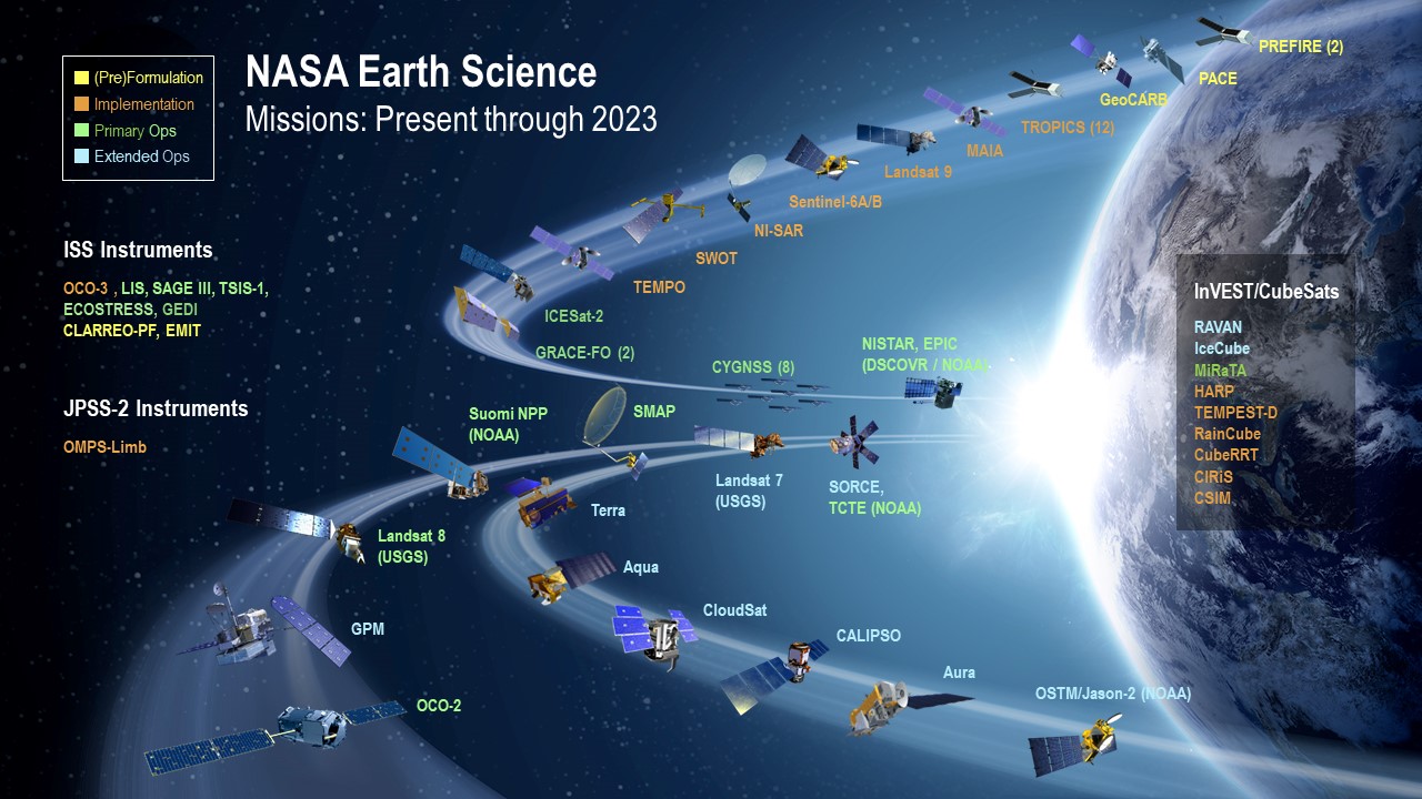
Unfortunately, this project cannot cover the entire list of Earth Observing Satellites (EOS) illustrated in the image. Nonetheless, NASA's missions and showcasing creditable sources for these data product is worth mentioning. Because of the vast missions and disciplinary categories, NASA must standardize the data products to ensure consistency throughout all missions. As shown in the image, this product will provide programming examples using the CYGNSS mission as the median to convey the concept.

The CYGNSS mission is to study the wind intensity of the hurricane/cyclone. As a result, its data products are managed by the Physical Oceanography Distributed Active Archive Center (PODAAC). The PODAAC is the custodian for gravity, ocean winds, sea surface temperature, ocean surface topography, sea surface salinity, and circulation disciplines. The PODAAC archives and manages the distributions of netCDF files for the earth science community and supports data from numerous missions that focus on the earth's oceans, atmosphere, cryosphere, and terrestrial hydrosphere. As a NASA data center, PODAAC provides access to data from both current and past missions, including satellite missions like CYGNSS, Jason-3, Sentinel-6, and Aquarius, among many others. The mission netCDF data products files are regularly updated and can be downloaded from the PODAAC website for scientific research and other applications. These data products are open to the public for researchers, educators, and hobbyists interested in earth science.
As mentioned in section 8.1, NASA's EOSDIS oversees Earth Science Data's life cycle and sets the standards for efficient production and stewardship of science-quality data. As a result, satellite data acquisition is segmented into data processing levels ranging from Level 0 to Level 4. The table below has been extracted from NASA's EOSDIS Data Processing Level website and has been modified to include the Author's footnote.
| Data Processing Levels | Description | Author's Footnotes |
|---|---|---|
| Level 0 | Reconstructed, unprocessed instrument and payload data at full resolution, with any and all communications artifacts (e.g., synchronization frames, communications headers, duplicate data) removed. (In most cases, NASA's EOS Data and Operations System (EDOS) provides these data to the DAACs as production data sets for processing by the Science Data Processing Segment (SDPS) or by one of the SIPS to produce higher-level products.) | L-0 data products are typically used by the manufacture/vendor to obtain calibration data and hardward specific data. It is uncommon to utilize this data unlesss the researcher has a desire to optimize the instrumentation. |
| Level 1A | Level 1A (L-1A) data are reconstructed, unprocessed instrument data at full resolution, time-referenced, and annotated with ancillary information, including radiometric and geometric calibration coefficients and georeferencing parameters (e.g., platform ephemeris) computed and appended but not applied to L0 data. | L-1 data products are considered raw pre-processed data from the sensor instrumentation. This data are typically information/values obtained from observation and is generated from the onboard sensor of the spacecraft. |
| Level 1B | Level 1B (L-1B) L1B data are L1A data that have been processed to sensor units (not all instruments have L1B source data). | |
| Level 1C | Level 1C (L-1C) L1C data are L1B data that include new variables to describe the spectra. These variables allow the user to identify which L1C channels have been copied directly from the L1B and which have been synthesized from L1B and why. | |
| Level 2 | Level 2 (L-2) Derived geophysical variables at the same resolution and location as L1 source data. | L2 data product are considered posted processed data made from the spacecraft. This data was created from L1 data product and had been processed onboard the spacecraft through its scientific algorithmn. Additionally, L2 data product would usually contain the spacecraft position, travel velocity, and the time stamp of the observatio. |
| Level 2A | Level 2A (L-2A) Data contains information derived from the geolocated sensor data, such as ground elevation, highest and lowest surface return elevations, energy quantile heights (“relative height” metrics), and other waveform-derived metrics describing the intercepted surface. | |
| Level 2B | Level 2B (L-2B) Data are L2A data that have been processed to sensor units (not all instruments will have a L2B equivalent). | |
| Level 3 | Level 3 (L-3) Variables mapped on uniform space-time grid scales, usually with some completeness and consistency. | L3 Data products contains are similiar to L2 data product; however, it prepackaged to allow the observation be mapped uniformally based on the space-time gride. Similarly, this data product is dervived from L2 data products. |
| Level 3A | Level 3 (L-3A) L3A data are generally periodic summaries (weekly, ten-day, monthly) of L2 products. | |
| Level 4 | Level 4 (L-4) Model output or results from analyses of lower-level data (e.g., variables derived from multiple measurements). | L-4 data products contains model results from lower-level data. This data product may not be avavilable for certain EOS. |
In this project, we will exploit CYGNSS L1 and L2 data products to demonstrate the netCDF library and plot the measurement data observed from the spacecraft. A list of resources is provided below to describe the standardization of netCDF files.
netCDF standardization hyperlinks:
This section aims to execute code and demonstrate the usefulness of two netCDF libraries. As mentioned in section 4.3.2, the netCDF4 and xarray libraries contain functions that allow programmers to manipulate the data product. Below are two code cells, the first containing an example of reading a netCDF file using the netCDF4 library and the second code cell displaying the netCDF data structure using the xarray library.
The netCDF file for CYGNSS must be downloaded and placed within this project's root directory folder. Please see the link below to download the CYGNSS SpaceCraft-3, L-1 data product from the PODAAC server. It is required to create an account to access the netCDF, the account is free, and the data products are open to the public. Please note that the data file is approximately 1 Gigabyte in size.
Hyperlink: PODAAC CYGNSS SpaceCraft-3, L1 data product
Note: xarray.xr makes it easy to quickly view the data format of a netCDL data type for development as demostrated below
After downloading and placing the netCDF file in the root directory, run the code cell below to read the netCDF file. If an error occurs, verify that the netCDF file is correctly placed within the root directory and see section 4.3.2 to confirm the installation of the netCDF libraries.
data = Dataset(r'cyg03.ddmi.s20220918-000000-e20220918-235959.l1.power-brcs.a31.d32.nc')
data
<class 'netCDF4._netCDF4.Dataset'>
root group (NETCDF4 data model, file format HDF5):
Conventions: CF-1.6, ACDD-1.3, ISO-8601
standard_name_vocabulary: CF Standard Name Table v30
project: CYGNSS
featureType: trajectory
summary: CYGNSS is a NASA Earth Venture mission, managed by the Earth System Science Pathfinder Program. The mission consists of a constellation of eight small satellites. The eight observatories comprise a constellation that measures the ocean surface wind field with very high temporal resolution and spatial coverage, under all precipitating conditions, and over the full dynamic range of wind speeds experienced in a tropical cyclone. The CYGNSS observatories fly in 510 km circular orbits at a common inclination of 35°. Each observatory includes a Delay Doppler Mapping Instrument (DDMI) consisting of a modified GPS receiver capable of measuring surface scattering, a low gain zenith antenna for measurement of the direct GPS signal, and two high gain nadir antennas for measurement of the weaker scattered signal. Each DDMI is capable of measuring 4 simultaneous bi-static reflections, resulting in a total of 32 wind measurements per second by the full constellation.
program: CYGNSS
references: Ruf, C., P. Chang, M.P. Clarizia, S. Gleason, Z. Jelenak, J. Murray, M. Morris, S. Musko, D. Posselt, D. Provost, D. Starkenburg, V. Zavorotny, CYGNSS Handbook, Ann Arbor, MI, Michigan Pub., ISBN 978-1-60785-380-0, 154 pp, 1 Apr 2016. http://clasp-research.engin.umich.edu/missions/cygnss/reference/cygnss-mission/CYGNSS_Handbook_April2016.pdf
processing_level: 1
comment: DDMs are calibrated into Power (Watts) and Bistatic Radar Cross Section (m^2)
creator_type: institution
institution: University of Michigan Space Physics Research Lab (SPRL)
creator_name: CYGNSS Science Operations Center
publisher_name: PO.DAAC
publisher_email: podaac@podaac.jpl.nasa.gov
publisher_url: http://podaac.jpl.nasa.gov
sensor: Delay Doppler Mapping Instrument (DDMI)
source: Delay Doppler maps (DDM) obtained from the DDMI aboard CYGNSS observatory constellation
version_id: 3.1
title: CYGNSS Level 1 Science Data Record Version 3.1
ShortName: CYGNSS_L1_V3.1
id: PODAAC-CYGNS-L1X31
netcdf_version_id: 4.3.3.1 of Dec 10 2015 16:44:18 $
history: Tue Sep 20 11:57:39 2022: ncks -O -a -dsample,0,172183,1 -L1 --cnk_dmn=sample,1000 --cnk_dmn=ddm,4 --cnk_dmn=delay,17 --cnk_dmn=doppler,11 /tmp/qt_temp.Eg8552 /tmp/qt_temp.BS8552
../../src/produce-L1-files/produce-L1-files production_1@cygnss-data-1.engin.umich.edu 3 2022-09-18 00:00:00 2022-09-19 00:00:00
platform: Observatory Reference: cyg3 (C-SCID=2B)
l1_algorithm_version: 3.1
l1_data_version: 3.2
lna_data_version: 2
nadir_ant_data_version: 17
nadir_sidelobe_mask_version: -1
zenith_ant_data_version: 13
ant_temp_version: 1
eff_scatter_2d_version: 4
eff_scatter_3d_version: 6
nbrcs_scatt_1d_version: 9
gps_eirp_param_version: 7
prn_sv_maps_version: 1
land_mask_version: 1
near_land_mask_version: 1
very_near_land_mask_version: 1
open_ocean_mask_version: 1
ddm_a2d_version: 1
milky_way_version: 1
fresnel_coeff_version: 1
brcs_uncert_lut_version: 3
ddma_les_sel_luts_version: 2
mean_sea_surface_version: 1
zenith_specular_ratio_gain_version: 19
zenith_calibration_params_version: 17
anomalous_sampling_periods_version: 1
noise_floor_correction_version: 9
zenith_sig_i2_q2_correction_version: 4
ddm_nbrcs_scale_factor_version: 6
eirp_scale_factor_version: 2
bin_ratio_qc_version: 1
per_bin_ant_version: 1
date_created: 2022-09-20T11:57:39Z
date_issued: 2022-09-20T11:57:39Z
geospatial_lat_min: -42.009N
geospatial_lat_max: 42.568N
geospatial_lon_min: 0.001E
geospatial_lon_max: 360.000E
time_coverage_resolution: P0DT0H0M1S
time_coverage_start: 2022-09-18T00:00:00.499261595Z
time_coverage_end: 2022-09-18T23:59:59.999261608Z
time_coverage_duration: P1DT0H0M0S
NCO: 4.4.4
dimensions(sizes): sample(172184), ddm(4), delay(17), doppler(11)
variables(dimensions): int32 sample(sample), int8 ddm(ddm), int16 spacecraft_id(), int8 spacecraft_num(), int8 ddm_source(), int8 ddm_time_type_selector(), float32 delay_resolution(), float32 dopp_resolution(), float64 ddm_timestamp_utc(sample), int32 ddm_timestamp_gps_week(sample), float64 ddm_timestamp_gps_sec(sample), float64 pvt_timestamp_utc(sample), int32 pvt_timestamp_gps_week(sample), float64 pvt_timestamp_gps_sec(sample), float64 att_timestamp_utc(sample), int32 att_timestamp_gps_week(sample), float64 att_timestamp_gps_sec(sample), int32 sc_pos_x(sample), int32 sc_pos_y(sample), int32 sc_pos_z(sample), int32 sc_vel_x(sample), int32 sc_vel_y(sample), int32 sc_vel_z(sample), int32 sc_pos_x_pvt(sample), int32 sc_pos_y_pvt(sample), int32 sc_pos_z_pvt(sample), int32 sc_vel_x_pvt(sample), int32 sc_vel_y_pvt(sample), int32 sc_vel_z_pvt(sample), int8 nst_att_status(sample), float32 sc_roll(sample), float32 sc_pitch(sample), float32 sc_yaw(sample), float32 sc_roll_att(sample), float32 sc_pitch_att(sample), float32 sc_yaw_att(sample), float32 sc_lat(sample), float32 sc_lon(sample), int32 sc_alt(sample), float32 commanded_sc_roll(sample), float32 rx_clk_bias(sample), float32 rx_clk_bias_rate(sample), float32 rx_clk_bias_pvt(sample), float32 rx_clk_bias_rate_pvt(sample), float32 lna_temp_nadir_starboard(sample), float32 lna_temp_nadir_port(sample), float32 lna_temp_zenith(sample), int32 ddm_end_time_offset(sample), float32 bit_ratio_lo_hi_starboard(sample), float32 bit_ratio_lo_hi_port(sample), float32 bit_ratio_lo_hi_zenith(sample), float32 bit_null_offset_starboard(sample), float32 bit_null_offset_port(sample), float32 bit_null_offset_zenith(sample), int32 status_flags_one_hz(sample), int8 prn_code(sample, ddm), int32 sv_num(sample, ddm), int32 track_id(sample, ddm), int8 ddm_ant(sample, ddm), float32 zenith_code_phase(sample, ddm), float32 sp_ddmi_delay_correction(sample, ddm), float32 sp_ddmi_dopp_correction(sample, ddm), float32 add_range_to_sp(sample, ddm), float32 add_range_to_sp_pvt(sample, ddm), float32 sp_ddmi_dopp(sample, ddm), float32 sp_fsw_delay(sample, ddm), float32 sp_delay_error(sample, ddm), float32 sp_dopp_error(sample, ddm), float32 fsw_comp_delay_shift(sample, ddm), float32 fsw_comp_dopp_shift(sample, ddm), int8 prn_fig_of_merit(sample, ddm), float32 tx_clk_bias(sample, ddm), float32 sp_lat(sample, ddm), float32 sp_lon(sample, ddm), float32 sp_alt(sample, ddm), int32 sp_pos_x(sample, ddm), int32 sp_pos_y(sample, ddm), int32 sp_pos_z(sample, ddm), int32 sp_vel_x(sample, ddm), int32 sp_vel_y(sample, ddm), int32 sp_vel_z(sample, ddm), float32 sp_inc_angle(sample, ddm), float32 sp_theta_orbit(sample, ddm), float32 sp_az_orbit(sample, ddm), float32 sp_theta_body(sample, ddm), float32 sp_az_body(sample, ddm), float32 sp_rx_gain(sample, ddm), float32 gps_eirp(sample, ddm), float32 static_gps_eirp(sample, ddm), float32 gps_tx_power_db_w(sample, ddm), float32 gps_ant_gain_db_i(sample, ddm), float32 gps_off_boresight_angle_deg(sample, ddm), float32 ddm_snr(sample, ddm), float32 ddm_noise_floor(sample, ddm), float32 ddm_noise_floor_corrected(sample, ddm), float32 noise_correction(sample, ddm), float32 inst_gain(sample, ddm), float32 lna_noise_figure(sample, ddm), int32 rx_to_sp_range(sample, ddm), int32 tx_to_sp_range(sample, ddm), int32 tx_pos_x(sample, ddm), int32 tx_pos_y(sample, ddm), int32 tx_pos_z(sample, ddm), int32 tx_vel_x(sample, ddm), int32 tx_vel_y(sample, ddm), int32 tx_vel_z(sample, ddm), float32 bb_nearest(sample, ddm), float32 fresnel_coeff(sample, ddm), float32 ddm_nbrcs(sample, ddm), float32 ddm_les(sample, ddm), float32 nbrcs_scatter_area(sample, ddm), float32 les_scatter_area(sample, ddm), int8 brcs_ddm_peak_bin_delay_row(sample, ddm), int8 brcs_ddm_peak_bin_dopp_col(sample, ddm), float32 brcs_ddm_sp_bin_delay_row(sample, ddm), float32 brcs_ddm_sp_bin_dopp_col(sample, ddm), float32 ddm_brcs_uncert(sample, ddm), float32 bb_power_temperature_density(sample, ddm), float32 zenith_sig_i2q2(sample, ddm), float32 zenith_sig_i2q2_corrected(sample, ddm), float32 zenith_sig_i2q2_mult_correction(sample, ddm), float32 zenith_sig_i2q2_add_correction(sample, ddm), int32 starboard_gain_setting(sample), int32 port_gain_setting(sample), float32 ddm_kurtosis(sample, ddm), int32 quality_flags(sample, ddm), int32 quality_flags_2(sample, ddm), int32 raw_counts(sample, ddm, delay, doppler), float32 power_analog(sample, ddm, delay, doppler), float32 brcs(sample, ddm, delay, doppler), float32 eff_scatter(sample, ddm, delay, doppler)
groups:
The code cell above performs a read function using the netCDF library dataset function to open the netCDF and store the data into a variable data. Noticed that two statements or variables are passed into the function containing the file name and character 'r'. The character 'r' in this function refers to mode r, indicating that the data is being accessed in read-only mode with no modification to the original netCDF file. Also, the code outputs the variable data shown in the output cell.
The code cell performs a read function using the xarray library open_dataset function to open the netCDF and stores the data into a variable ds. Unlike Approach# 1, the function only requires one parameter to be passed into the function, which is the file name. By default, this function opens the netCDF with read-only access.
ds = xr.open_dataset('cyg03.ddmi.s20220918-000000-e20220918-235959.l1.power-brcs.a31.d32.nc')
ds
<xarray.Dataset>
Dimensions:                          (sample: 172184, ddm: 4, delay: 17,
                                      doppler: 11)
Coordinates:
  * sample                           (sample) int32 0 1 2 ... 172182 172183
  * ddm                              (ddm) int8 0 1 2 3
    ddm_timestamp_utc                (sample) datetime64[ns] ...
    sp_lat                           (sample, ddm) float32 ...
    sp_lon                           (sample, ddm) float32 ...
Dimensions without coordinates: delay, doppler
Data variables: (12/126)
    spacecraft_id                    int16 ...
    spacecraft_num                   int8 ...
    ddm_source                       int8 ...
    ddm_time_type_selector           int8 ...
    delay_resolution                 float32 ...
    dopp_resolution                  float32 ...
    ...                               ...
    quality_flags                    (sample, ddm) float64 ...
    quality_flags_2                  (sample, ddm) float64 ...
    raw_counts                       (sample, ddm, delay, doppler) float64 ...
    power_analog                     (sample, ddm, delay, doppler) float32 ...
    brcs                             (sample, ddm, delay, doppler) float32 ...
    eff_scatter                      (sample, ddm, delay, doppler) float32 ...
Attributes: (12/66)
    Conventions:                          CF-1.6, ACDD-1.3, ISO-8601
    standard_name_vocabulary:             CF Standard Name Table v30
    project:                              CYGNSS
    featureType:                          trajectory
    summary:                              CYGNSS is a NASA Earth Venture miss...
    program:                              CYGNSS
    ...                                   ...
    geospatial_lon_max:                   360.000E
    time_coverage_resolution:             P0DT0H0M1S
    time_coverage_start:                  2022-09-18T00:00:00.499261595Z
    time_coverage_end:                    2022-09-18T23:59:59.999261608Z
    time_coverage_duration:               P1DT0H0M0S
NCO: 4.4.4In this example, the netCDF data can be accessed via the variables data and ds imported from the netCDF and xarray libraries, respectively. By observation, the xarray library provides a much more structured and readable dataset when the ds variable is displayed output in HTML format. Consequently, the netCDF library provides a much more friendly approach and useability for its function calls. As a result, this project will use the xarray library only to read the header file of the netCDF file, and the netCDF library will be used to exploit the data product. Even though this approach is redundant, it illustrates the usability of libraries and demonstrates multiple options to solve a problem.
As demonstrated in the ds output, the metadata prints the details for the CYGNSS L1 data product. This particular netCDF file follows the Hierarchical Data Formats (HDF-5) standards. HDF files are multi-dimensional array file groups organized in a specific data structure. The image below shows that HDF5 data is organized similarly to a parent and child folder structure with metadata to describe each group.
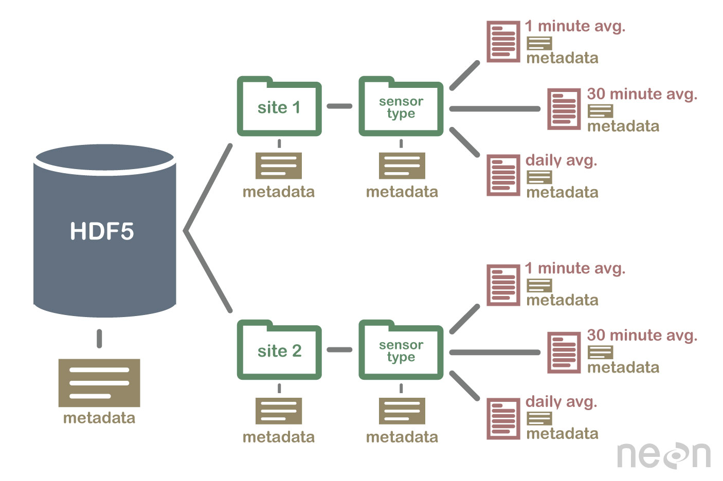
Note: For more information regarding HDF see, Intro to HDF
In this example, the variable ds shows that the netCDF file contains a multiply-dimension array file formation with 172184 samples. Moreover, variables such as the spacecraft's coordinates, data variables, and instrumentation sensor, Delayed Doppler Map (DMM) are described within the metadata. Furthermore, the type cast of the data variable is also described in the metadata, indicating where the data structure is an integrator, float, etc.
This section will provide three examples demonstrating the procedures to extract data from the netCDF file for analysis. Like the examples in the paragraphs above, we will run the code and then explain each instance. The examples provided in this section are as follows:
Before diving into the code, I recommend constantly referring to the printout display offered by the xarray library in section 8.3. The image below shows that the xarray dataset contains a data structure group, Data Variables. A drop-down arrow, highlighted in yellow, is used to expand the list. Furthermore, highlighted in green, the attribute menu expands and describes the data values. Lastly, the data report attribute, highlighted in blue, provides insight into the typecast for the variable.
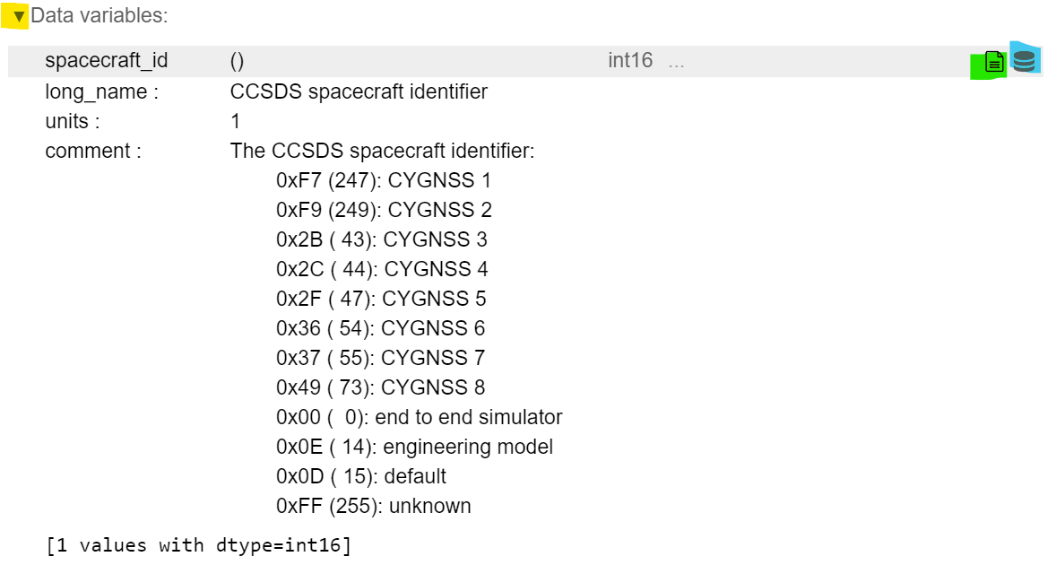
CYGNSS is an eight-constellation satellite system; it is essential to know which satellite data is analyzed. In this example, we will execute the code cell below and determine which of the eight satellite data collections is recorded within this netCDF file.
Note: Select the code cell below and run the code. If an error occurs, please refer to section 7 to verify that libraries code has been correctly executed.
spacecraft_id = data.variables['spacecraft_id']
print(spacecraft_id[0])
print(spacecraft_id[172183])
43
43
The code cell output shows the value 43 printed twice. The spacecraft variable is accessible through the netCDF library class. The code statement data.variables['spacecraft_id'] is a class function call that extracts the values from the netCDF files for the spacecraft and stores it in the spacecraft_id variable. The variable spacecraft_id is an array of 172184 elements containing int16 data products. In this example, a print statement of array elements 0 and 172183 is printed to demonstrate that the spacecraft is consistent throughout the entire file. The value 43 corresponds to the hexadecimal 0x2B and CYGNSS satellite number 3. Furthermore, the file name provides insight validating that the output value is 43. The file name below shows that the nomenclature, cyg03, instantiates CYGNSS satellite number 3.
Filename: cyg03.ddmi.s20220918-000000-e20220918-235959.l1.power-brcs.a31.d32.nc
| Nomenclature | Descripition |
|---|---|
| cyg03 | CYGNSS Satellite 3 |
| ddmi | Delay Doppler Map Instrument |
| s20220918-000000-e20220918-235959 | Collected Data from Sensor Instrumentation, Starting 09.18.22 at 000000 and Ending 09.18.22 at 235959 |
| l1 | Data Product L-1 |
| .nc | netCDF file |
Another vital aspect contained in a netCDF is spatial information. This section provides an example of extracting essential longitudinal, latitudinal, and altitudinal data for earth scientists to conduct analysis.
Note: Select the code cell below and run the code. If an error occurs, please refer to sections 7 and 8.3 to verify that libraries code has been correctly executed.
#Space Craft longitude and array size/points
lon = data.variables['sc_lon'][:]
print ("SC Longitude:")
print (lon)

lon_len = len(lon)
print ("Longitude elements:")
print (lon_len)

#Space Craft lattitude and array size/points
lat = data.variables['sc_lat'][:]
print ("SC Lattitude:")
print (lat)

lat_len = len(lat)
print ("Lattitude elements:")
print (lat_len)

#Space Craft Alttitude and array size/points
alt = data.variables['sc_alt'][:]
print ("Space Craft Altitude:")
print (alt)

alt_len = len(alt)
print ("Altitude elements:")
print (alt_len)
SC Longitude:
[114.76621 114.79587 114.82552 ... 169.28778 169.31303 169.33829]
Longitude elements:
172184
SC Lattitude:
[ 25.433258  25.419817  25.40639  ... -12.998617 -13.015864 -13.03311 ]
Lattitude elements:
172184
Space Craft Altitude:
[512302 512298 512289 ... 507331 507333 507338]
Altitude elements:
172184
The code cell output shows the value for the spacecraft's longitudinal data in lines 1-4, latitudinal data in lines 10-13, and altitudinal information in lines 24-26. In this example, code lines 1-4 show the syntax in [:] indicating that the entire sc_lon matrix be stored in the variable lon. The printout for the lon variable is a matrix containing a long list of longitude data. Furthermore, the code for matrix length (len) returns a value emphasizing the element within the matrix. As shown in lines 6-8, the longitudinal data contains 172184 elements, as expected. The code lines 1-4 were repeated to extract latitude and altitude information as shown in the code cell printout statement.
Equally important is the time stamp data observed and collected by the instrumentation onboard the spacecraft. This section provides an example of interpolating the time stamp artifact and translating the time into standard clock time format. This statement aligns with the nomenclature discussed in section 8.4.1.
Note: Select the code cell below and run the code. If an error occurs, please refer to sections 7 and 8.3 to verify that libraries code has been correctly executed.
#System time UTC
time = data.variables['ddm_timestamp_utc'][:]
time_len = len(time)
print (time[0])
print (time[1])
print (time[10])
print (time_len)
0.0
0.500000039
4.999999948
172184
The code cell output shows the time value stored in the variable time. According to the xarray HTML metadata display shown below, the ddm_timestamp_utc represents the time coverage from the Delay Doppler Map (DDM) instrumentation/sensor. Highlighted in yellow are indications that the time stamp is within Universal Time Coordinate (UTC) format with nanosecond resolution. Furthermore, UTC is also referred to as Zulu time by the Military.
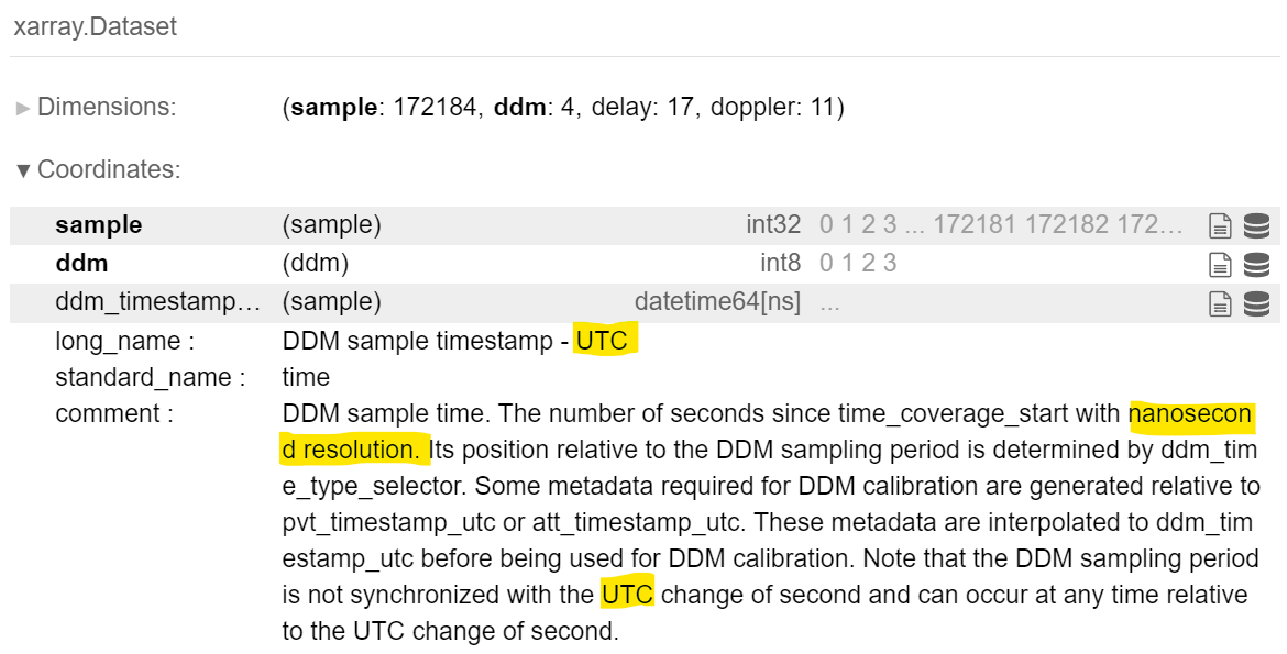
As shown in the code cell print, the matrix time index at 0, time [0] outputs a value of 0 seconds. Meanwhile, the matrix time index at 1, time [1] is 0.500000039, showing nine decimal precision and validating the precision of the time recorded is within nanosecond accuracy.
Up to this point in the project, the example discussion topics were limited to software. From this point forward, the data product and discussion will be more influenced by the physicality, science, and operational conditions of CYGNSS.
For example, the CYGNSS handbook pg.42 mentions that the time stamps update are of 1 Hz increments. Furthermore, the netCDF metadata description is also misleading, referencing the time stamp incrementally by nanosecond resolution. The CGYNSS handbook and netCDF metadata need to be more accurate, but with some intuition and logic, the timestamp can be revealed its secrets.
The CYGNSS handbook suggests the timestamp for L-1 data products are generated at 1 Hz intervals, yielding a sampling rate of 1 data product per second. Mathematically, a 1 Hz sampling rate will produce 24ℎ𝑟𝑠∗60𝑚𝑖𝑛𝑠∗60𝑠𝑒𝑐𝑠 = 86400 data points. Furthermore, the netCDF metadata suggested (10^9) resolution yielding 24ℎ𝑟𝑠∗60𝑚𝑖𝑛𝑠∗60𝑠𝑒𝑐𝑠∗ 10^9 𝑟𝑒𝑠𝑜𝑙𝑢𝑡𝑖𝑜𝑛= 8.64∗10^13 data points. Therefore, the metadata description and CYGNSS handbook provide misleading information and do not resemble the data samples 172,184 datapoints within this example.
Although both resources can be misleading, the metadata file description and CYGNSS handbook provide some of the truth and hint at 172,184 datapoints. As shown in the code cell print state of the variable time index at 0, 1, and 10, the timing values for the DDM time at 0 are 0.500000039 seconds and 4.999999948 seconds, respectively. These two values correspond to the nanosecond metadata descriptors; however, they are misleading as the sampling rate is not of nanosecond incremental resolution. Furthermore, the handbook mentions that the sampling rate is 1 Hz, but the example shows that the sampling rate is closer to 2 Hz. As a result, the mathematical formula for a 2 Hz sampling rate yields 2Hz ∗ 60𝑠𝑒𝑐 ∗ 60𝑚𝑖𝑛𝑢𝑡𝑒𝑠 ∗ 24ℎ𝑟𝑠 = 172800 data points. The data points are close to the sample value of 172184, as described in the variable time_len. The discrepancy between 172,184 and 172,800 data points are expected as the data is factual information; an outage can occur, timing can be delayed, noise, rounding error, etc.
It is essential to realize that this example provides a bit of intuition to analyze the data product. The netCDF L-1 data product file was published in Sept 2022, and the handbook was published in April 2016. Over six years have passed since the handbook was revised and improved, and a series of improvements must have occurred to increase the sensor instrumentation sampling rate from 1 Hz to 2 Hz. Nevertheless, realizing that the data analyzed is actual data obtained within operational conditions and not theoretical data is essential.
Another essential aspect is converting the sampling interval time to a standard time format. As mentioned in the previous paragraphs, the time variable is a matrix of 172184 elements, and the elements are incremented by 0.5 seconds with nanosecond resolution. Therefore, we can assume that time[122] will yield 62 seconds rather than 00:00:01:01 (HH:MIN: SEC), displayed in Military ZULU time. Before is a code cell containing a function to convert seconds into standard time format, making it easier to determine the hour and time of the day. Immediately following the code cell with function code, a code cell below was created to experiment with a different element of the time matrix by changing the value x.
Note: Select the code cell below and run the code. If an error occurs, please refer to sections 7 and 8.3 to verify that libraries code has been correctly executed.
def convert_seconds(seconds):
    seconds = seconds % (24 * 3600)
    hour = seconds // 3600
    seconds %= 3600
    minutes = seconds // 60
    seconds %= 60
    return "%d:%02d:%02d" % (hour, minutes, seconds)
x = 123
sample_time = convert_seconds(time[x])
print(sample_time)
0:01:01
As shown in the first code cell, python requires a function to be defined using the reserved word "def." Immediately following the term "def" is the name of the function and the variables surrounded by parentheses. In this case, a variable name seconds is surrounded by parentheses and is used in the function to calculate and derive seconds into standard time format. Also, noticed that a colon ":" and tab are required to create the function. Please see the explanation by Jayant Verma, for details regarding the algorithm.
It is important to notice that when x = 120, the sample time output is 00:00:59 rather than 00:01:01. Furthermore, the sample time outputs 00:01:01 when the x is 123. This discrepancy may be due to timing delay, noise, rounding error, etc. Again, the data product analyzed is actual data and not theoretical data.
In summary, this section provided detailed examples of extracting L-1 data products for analysis. Data such as spacecraft identification number, spatial information (lat/long/alt), and time stamp information was obtained with just a few line of code. The function convert_seconds will be used in the L-2 data product Jupyter Notebook.
Section 8.0 provided a detailed guide to extracting L-1 Data products. The next logical step is to plot the data products on a map and generate visual aids helpful for scientists/analysts to present their earth science idea and discovery. In addition to the libraries previously used, this section will utilize several new libraries, such as cartopy and matplotlib. Moreover, the examples will also use the same netCDF file discussed in previous sections. This section will provide two examples:
It is essential to understand that the methods used in this example are imperfect and have one limitation. The limitation discovered using this method is not being able to discriminate altitude. As a result, the maps generated using this method are in 2-D plots. Unlike Google Earth, cartopy is unable to create 3-D views and perspectives. Although some may see this feature as a limitation, the need for 3-D representation may not be required. Nonetheless, using the cartopy library provides a method to generate maps with very little code, requires minimum computation power, and generates plots relatively quickly. For more information regarding the cartopy library, please see the link below.
Useful hyperlink: cartopy
In addition to the libraries used in previous sections, matplotlib and cartopy library functions are used to generate a map. Generating a map is relatively simple, requiring only five lines of code within this example.
Note: Select the code cell below and run the code. If an error occurs, please refer to all the code in previous sections.
fig = plt.figure(figsize=(16, 20))
fig = plt.axes(projection=ccrs.Robinson(0))

fig.stock_img()

# Save the plot by calling plt.savefig() BEFORE plt.show()
#plt.savefig('Robinson_Map_Projection.pdf')
#plt.savefig('Robinson_Map_Projection.png')

fig.plot(lon, lat, color='orange', transform=ccrs.Geodetic())
plt.show()
As mentioned in section 8.4.2, the longitudinal and latitudinal data was obtained from the CYGNSS L-1 data product and stored in the variables lon and lat. In this example, the cartopy library function call transforms the spatial information into x and y coordinates using matplotlib to plot the spatial data on a Geodetic projection accurately. Provided below is a procedural explanation for the code required to generate the map.
1: The line plt.axes(projection=ccrs.PlateCarree()) sets up a GeoAxes instance which exposes a variety of other projections. click here for a list of projection.
2: The value "0" represents the central longitude projection of the map. This number can be modifed to a value that ranges between -180 to +180 degrees to rotate the center longitude of the map.
3: The core concept is that the projection of your axes is independent of the coordinate system your data is defined in. The projection argument is used when creating plots and determines the projection of the resulting plot (i.e. what the plot looks like). The transform argument to plotting functions tells Cartopy what coordinate system your data are defined in.
Section 9.1 provided a straightforward approach to generate a map and plot L1 data products; however, the Robinson projection lacks vital information such as (lat/lon) axes labels and specific features. CYGNSS L1 data product will be plotted on a PlateCarree global map projection in this example. This example will demonstrate methods to include features, such as creating axis labels and adding map features.
Note: Select the code cell below and run the code. If an error occurs, please refer to all the code in previous sections.
# Add Figure with Size of the Figure
fig2 = plt.figure(figsize=(20, 24))

# Add Map Projection
fig2 = plt.axes(projection=ccrs.PlateCarree())

# Add Map Features
fig2.add_feature(cfeature.LAND)
fig2.add_feature(cfeature.COASTLINE)
fig2.add_feature(cfeature.OCEAN)
fig2.add_feature(cfeature.BORDERS, linestyle=':')
fig2.add_feature(cfeature.LAKES, alpha=0.5)
fig2.add_feature(cfeature.RIVERS)
fig2.stock_img()

#Add Latitude and Longitude Labels
grid_lines = fig2.gridlines(draw_labels=True)
grid_lines.xformatter = LONGITUDE_FORMATTER
grid_lines.yformatter = LATITUDE_FORMATTER

#Add Legend to Map
fig2.plot(lon, lat, color='green', transform=ccrs.Geodetic(), label='CYGNSS-3')
fig2.legend()

plt.show()
Unlike the example in section 9.1, this example provides a map that contains spatial coordinates, certain map features, and CYGNSS L-1 data products plotted in green. Moreover, the variable name has changed from fig to fig2 to help distinguish the difference between examples. Provided below is a procedural explanation for the code required to generate the map:
Line 2: Using matplotlib to create a new figure of a specific width x height (20inches x 24inches) and store the figure in the variable fig2.
Line 5: Generate a map projection, then set the plot to a variable1 2 3
Lines 8-14: Add features to the map and overlay artist drawing using axis.stock_img()4
Line 17-19: Add Latitude and Longitude coordinate labels using the cartopy.grider library function, then formate the figure's x-axis as longitude and y-axis as latitude. The statement "True" can be modified to "False" to remove the lat/lon gride lines.
Line 22: Transform the netCDF Spacecraft position (lon,lat) values into a geodetic (WGS84 globe coordinate) information ready for plotting. Also, modify the plot data color green and add a label to the plot.
Line 23: Add legend to map5
Line 25: Display the map and L1 data product plot by executing plt.show()
1: The line plt.axes(projection=ccrs.PlateCarree()) sets up a GeoAxes instance which exposes a variety of other projections. click here for a list of projection.
2: The core concept is that the projection of your axes is independent of the coordinate system your data is defined in. The projection argument is used when creating plots and determines the projection of the resulting plot (i.e. what the plot looks like). The transform argument to plotting functions tells Cartopy what coordinate system your data are defined in.
3: The value "0" represents the central longitude projection of the map. This number can be modifed to a value that ranges between -180 to +180 degrees to rotate the center longitude of the map.
4: The caropy library has plenty of map features that can be used for many different needs. For a list of map features click here.
5: Noticed that the legend will appear by default in the upper right hand corner according to the characterstics (color, line, etc) set from the plot. click here.
Although the examples in sections 9.1 and 9.2 have laid the general foundation to create maps useful to the earth science community, these examples are intended to introduce cartopy and matplotlab libraries briefly. The next logical step in this project is to create an animated plot and bind the example to a real-life and relevant catastrophe.
In this example, the matplotlib animation library function call is deployed to generate an animated map. Although the nomenclature for the L-1 Data product was discussed in section 8.4.1, the date for the file name has a significant value. The file name contains the date 09.18.2022 marking the date for Hurricane Fiona.
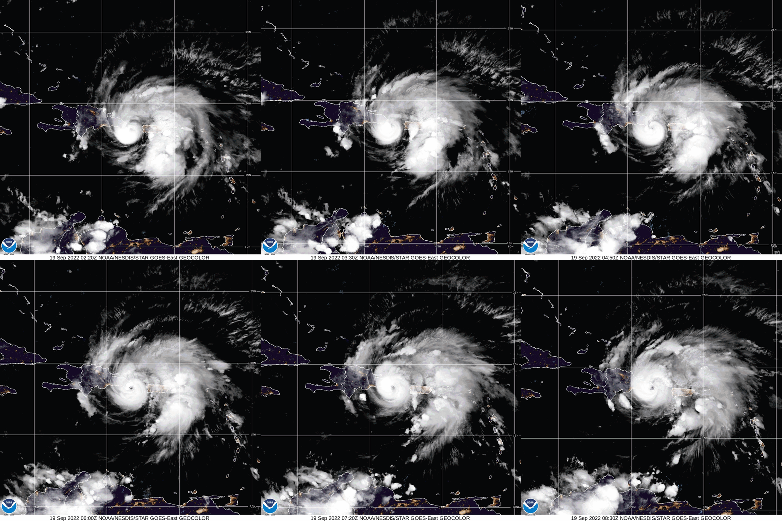
Hurricane Fiona was a large and powerful storm with destructive Category-4 winds. The National Oceanic and Atmospheric Administration (NOAA) began tracking this hurricane on September 14-18, 2022. On September 19, 2022, Hurricane Fiona made landfall on the coast of Pureto, killing at least four people and leaving the island without power.
Note: Select the code cell below and run the code. If an error occurs, please refer to all the code in previous sections. Simulation of the map per minute interval may take more than 30mins to execute. After completing the simulation, run the markdown cell below the code cell to open the save animated plot.
#User must enter date below: Mon DD YY
MM = "Sep"
DD = 18
YY = 2022

#User to must specify plotting rate, True or False
Per_hour = False

# Add Figure with Size of the Figure
fig3 = plt.figure(figsize=(16, 20))

# Add Map Projection
fig3 = plt.axes(projection=ccrs.PlateCarree())

# Add Map Features
fig3.add_feature(cfeature.LAND)
fig3.add_feature(cfeature.COASTLINE)
fig3.add_feature(cfeature.OCEAN)
fig3.add_feature(cfeature.BORDERS, linestyle=':')
fig3.add_feature(cfeature.LAKES, alpha=0.5)
fig3.add_feature(cfeature.RIVERS)
fig3.stock_img()

#Add Latitude and Longitude Labels
grid_lines = fig3.gridlines(draw_labels=True)
grid_lines.xformatter = LONGITUDE_FORMATTER
grid_lines.yformatter = LATITUDE_FORMATTER

#Add the initial point at UTC zero
[point] = fig3.plot(lon[0], lat[0], marker='$3$', markersize=15, color='red', transform=fig3.projection, label='CYGNSS-3')

#Adding Plotting
fig3.plot(lon, lat, transform=ccrs.Geodetic(), color='gray')

#Add Plot Specifics
fig3.set_title('CYGNSS Orbit Plot')
fig3.legend()

#Configure Date
MM = str(MM)
DD = str(DD)
YY = str(YY)
date = MM + " " + DD + ", " + YY + " "

#Variables reserved for setting up animation frame
secs = 2
mins = 60*secs
hrs= 60*mins

if (Per_hour):
    timescale = hrs
    frame = 24
    interv = 1000
else:
    timescale = mins
    frame = 1434
    interv = 100

#Animatation function
def animate_point(i):

    #animate plot title to display calendar and clock
    military_time = convert_seconds(time[i*timescale])
    military_time = str(military_time)
    date_time = date+military_time
    fig3.set_title(date_time, fontsize=40, color='black', fontweight='bold')

    #animate plot with the location of CYGNSS
    point.set_data(lon[i*timescale], lat[i*timescale])

anim = FuncAnimation(fig3.figure, animate_point, frames=(frame), interval=interv)

#Save Animation
anim.save('LAT_LON_CYGNSS_3.gif', writer='imagemagick')

HTML(anim.to_jshtml())
MovieWriter imagemagick unavailable; using Pillow instead.
C:\Users\Snow White\AppData\Local\Temp\ipykernel_23912\2951397505.py:69: MatplotlibDeprecationWarning: Setting data with a non sequence type is deprecated since 3.7 and will be remove two minor releases later
  point.set_data(lon[i*timescale], lat[i*timescale])
C:\Users\Snow White\AppData\Local\Temp\ipykernel_23912\2951397505.py:69: MatplotlibDeprecationWarning: Setting data with a non sequence type is deprecated since 3.7 and will be remove two minor releases later
  point.set_data(lon[i*timescale], lat[i*timescale])

The example above shows that the CYGNSS L-1 data product provides the spatial information necessary to plot the third satellite's position. The map animates satellite 3 orbiting the earth and displaying its position in minute or hour increments. By observation, the satellite's ground track travels fast, giving only a short window of opportunity to observe the hurricane. Imagine the constellation of eight satellites, the chance to observe a storm like Hurricane Fiona increases traumatically. Due to the time it takes to run the code; this example allows the user to generate an animated map in hours or minute increments. Provided below is a procedural explanation for the code required to generate the animated map:
Line 10: Using matplotlib to create a new figure of a specific width x height (16inches x 20inches) and store the figure in the variable fig3.
Line 13: Generate a map projection, then set the plot in variable fig3 variable 1 2 3
Lines 16-22: Add features to the map and overlay artist drawing using axis.stock_img()4
Lines 25-27: Add Latitude and Longitude coordinate labels using the cartopy.grider library function, then formate the figure's x-axis as longitude and y-axis as latitude. The statement "True" can be modified to "False" to remove the lat/lon gride lines.
Line 30: Set the initial plotting point starting at position 0. Afterwards, add features for the animated moving icon such as the symbol, color, and size. Setting the points to zeroth index is necessary as the value will be incremented using the animated function.
Optional, Line 32: Transform the netCDF Spacecraft position (lon,lat) values into a geodetic (WGS84 globe coordinate) information ready for plotting. This is done to keep a track of the flight trajectory of the moving dot.
Line 36: Add Title for the Figure
Line 37: Add legend to map5
Lines 40-43: Creates a string variable to contain the map's title.
Lines 46-57: Sets the parameters required for animation. For examples, the variable secs is set to 2 because CYGNSS L1 data record its observation at 2Hz. Moreover, the if statement contains the logic to generate the animation according to the user perference of hour or minute increment animation.
Lines 60-69: A function, animate_point is created to generate the animation. This function will incrementally (lat/lon) index according to the point variables mentioned in step 5. Additionally the date with time will increment according to the boolean flag set by the user. This boolean flag will specify where the animation generated will represent hours or minutes intervals. This function will loop according to the on FuncAnimation parameters.5 6
Line 71: Set the parameters for FuncAnimation. The arguements passed in this function is the figure used to get needed events callable function, frames or interation, and intervals (delay in milliseconds between consecutive animation runs)
Line 74: Saves the animation according the filename, Lat_Long_CYGNSS3.gif. 7
Line 76: Jupyter notebook is a server to client python IDE and unfortunately have some limitations. A limitation in Jupyter notebook is that it currently does not fully support html animation. Line 76 is a work around solution for this limitation.
1: The line plt.axes(projection=ccrs.PlateCarree()) sets up a GeoAxes instance which exposes a variety of other projections. click here for a list of projection.
2: The core concept is that the projection of your axes is independent of the coordinate system in your data defined. The projection argument is used when creating plots and determines the projection of the resulting plot (i.e., what the plot looks like). The transform argument to plotting functions tells Cartopy what coordinate system your data are defined in.
2: The value "0" represents the central longitude projection of the map. This number can be modified to a value that ranges between -180 to +180 degrees to rotate the center longitude of the map.
3: Notice that the variable changed from ax (axis) to map. Both are used interchangeably to denote that both x and y axis must be defined to generate a map. We will be using m denoting map moving forward throughout this program.
4: Noticed that the legend will appear by default in the upper right-hand corner according to the characteristics (color, line, etc.) set from the plot. click here
5: Noiced that seconds is multipled by 2. CYGNSS data for DMM time is measured by every half-second interval with the accuracy of 1ns per sample. The handbook is misleading. Also, the parameters for the animation, defined as timescale, frame, and interv, are important aspects of the animation. Starting with the simplest variable interv, represents the millisecond interval or delay between each image. Furthermore, the variable timescale represents the index for the L1 data product. Lastly, the frame represents the number of frames within the animation or increments of the variable i.
6: The constant 1432 is unique to this particular data file. Recall that the netCDF file contained 172184 elements, and the theortical maximum data point should be (2 60 60 * 24) = 172200. Hence, (172184/2) = 86092 seconds and (86092/60) = 1434.86 minutes. As a result, the frames required are 1434 frames/minute.
7: The library matplotlib supports multiple file formats such as png, jpeg, gif, ppm, etc. Also supported is the creation of video files. For more information click here
With the examples provided within this volume, a scientist of any programming skill level should have the fundamental knowledge to plot and map L-1 data products of any EOS mission orbiting the earth as illustrated in the image below. Although frustrating, debugging a code error is part of the software development cycle and may take many hours to resolve. This process is an investment of time to practice and become better at a skill set that will pay huge future dividends.
This volume provided the essential process to map and generate plots based on netCDF with multiple uses and a demonstration of several libraries. Some examples are straightforward and have no actual application but provide the necessary concept. These examples led to the building blocks required to demonstrate these concepts with real-life applications and show coordination with current events such as Hurricane Fiona.
Again, this volume provides an introduction and several examples to demonstrate the concept. Unfortunately, the L-1 data product only provides raw data extracted from the onboard sensor instrumentation, as referenced in section 8.2. Post-processing of L-1 data products is required to obtain the wind speed information observed by the spacecraft. To acquire wind speed, scientists have two options: 1. Generate your algorithm to calculate the wind speed from the L-1 raw data product, or 2. Utilize the L-2 data product and trust that CYGNSS onboard algorithm calculation is sufficient to calculate the wind speed observed at the specular point.
As a result, this volume did not dive deep into the science of microwave remote sensing theory or the science of CYGNSS. The intent was to provide detailed examples to enable scientists to generate maps and plots quickly. The next volume will cover L-2 data products, the science of CYGNSS, and microwave remote sensing in greater detail.